[Notes] CSCI 567 ML lec1 KNN and ML system

21 Jan 2020 | CSCI567, English/英文, Note

Credit to: Prof. Yan Liu, CSCI567, Spring 2020

Outline

• Course Overview
• ML overview
• General setup for multi-class classification
• Nearest Neighbor Classifier (NNC)
• Some theory NNC

---

One possible definition

A set of methods that can automatically detect patterns in data, and then use the uncovered patterns to predict future data, or to perform other kinds of decision making under uncertainty

Key ingredients in ML

• Data collected from past observation (often training data)
• Modeling devised to capture the pattern in the data. “All models are wrong, but some are useful” - George Box
• Prediction apply the model to forecast what is going to happen in future.

Different flavor of learning problems

• Supervised learning Aim to predict
• Unsupervised learning Aim ti discover hidden and latent patterns and explore data
• Reinforcement learning Aim to act optimally under uncertainty

Distinguish between AI and ML *

• ML Tools of learning problems SVN, decision tree …
• AI How to in design a intelligence agent. Bigger set. Planning, control, and traditional image recognition and natural language processing usually is part of AI and not part of ML
• DS Focus on application

General setup for multi-class classification

• Data: N samples/instances \(D^{\text{TRAIN}}={(\boldsymbol{x_1},ay_1),(\boldsymbol{x_2},y_2), ..., (\boldsymbol{x_N}, y_N)}\)
  • $\boldsymbol{x_n}\in \mathbb{R}^D$ is called a feature vector
  • $y_n\in [C] = {1,2,…,C}$ is called a label/class/category
  • Used to learn future prediction function $f:\mathbb{R}^D \rightarrow[C]$

  when $C=2$, it is binary classification

Nearest Neighbor Classification (NNC)

It is pretty good classifier, the problem is to define the distance/similarity of cases

\[\boldsymbol{x}(1) = \boldsymbol{x}_{\text{nn}(\boldsymbol{x})}\]

where $\boldsymbol{x}(1)$ means the nearest 1 neighbor, $\text{nn}(\boldsymbol{x})\in [N]={1,2,…,N]}$ is the label of given feature vector $\boldsymbol{x}$

\[\text{nn}(\boldsymbol{x})=\arg\min _{n\in[N]}\|\boldsymbol{x}-\boldsymbol{x}_n\|_2=\arg\min_{n\in[N]} \sqrt{\sum^D_{d=1}(x_d-x_{nd})^2}\]

where $|\cdot|_2$ is the $L_2$ (i.e. Euclidean distance, because that is easy, smooth)

Classification rule: $y=f(\boldsymbol{x})=y_{\text{nn}(\boldsymbol{x})}$

Other Distances

• $L_1$ distance (i.e. Manhattan distance)

  \[\|\boldsymbol{x}-\boldsymbol{x}_n\|_1 = \sum^D_{d=1}|x_d-x_{nd}|\]

• Generally, $L_p$ distance (for $p\ge 1$)

  \[\|\boldsymbol{x}-\boldsymbol{x}_n\|_p = (\sum^D_{d=1}|x_d-x_{nd}|^p)^{1/p}\]

  when $p\rightarrow \infty$ means choosing the maximum difference

Decision Boundary

Determine the label of every point in the space a decision boundary that partitions the space into different regions will rise. It is used to observe a known function. (hard to draw when the function is unknown)

Metric for Performance Evaluation

• accuracy

  \[A^\text{TEST}=\frac{1}{M}\sum_m\mathbb{I}[f(\boldsymbol{x}_m)==y_m]\]

• error rate

  \[\varepsilon^\text{TEST} = \frac{1}{M}\sum_m\mathbb{I}[f(\boldsymbol{x}_m)\neq y_m]\]

where $\mathbb{I}[\cdot]$ is the indicator function. e.g. $\mathbb{I}[\text{true}]=1$, $M$ is the number of test cases.

K-Nearest Neighbor (KNN)

• 1-nearest neighbor:

  \[\text{nn}_1(\boldsymbol{x})=\arg\max_{n\in[N]}\|\boldsymbol{x}-\boldsymbol{x}_n\|_2\]

• 2-nearest neighbor:

  \(\text{nn}_2(\boldsymbol{x})=\arg\max_{n\in[N]-\text{nn}_1(\boldsymbol{x})}\|\boldsymbol{x}-\boldsymbol{x}_n\|_2\) (label of second nearest neighbor)

The set of K-nearest neighbor:

\[\text{knn}(\boldsymbol{x})=\{\text{nn}_1(\boldsymbol{x}),\text{nn}_2(\boldsymbol{x}),..., \text{nn}_K(\boldsymbol{x})\}\]

with $\boldsymbol{x}(k)=\boldsymbol{x}_{\text{nn}_k(\boldsymbol{x})}$ we have, (distence to the first nearest neighbor is smaller then the second nearest neighbor …)

\[\|\boldsymbol{x}-\boldsymbol{x}(1)\|_2^2\le\|\boldsymbol{x}-\boldsymbol{x}(2)\|_2^2\le ... \le \|\boldsymbol{x}-\boldsymbol{x}(K)\|_2^2\]

Classify with K neighbors

Every neighbor vote and pick the majority. There can be many ways to do that e.g. weighted vote, take simple majority with odd number of neighbors, etc.

\[y=f(\boldsymbol{x})=\arg\max_{c\in [C]} \sum_{n\in \text{knn}(\boldsymbol{x})}\mathbb{I}(y_n==c), \forall c\in[C]\]

Preprocessing data

issue: distance depend on units of the features solution: preprocess data, “normalized”

one example:

• mean:

  \[\bar{x}_d=\frac{1}{N}\sum_nx_{nd}\]

• standard deviations:

  \[s^2_d=\frac{1}{N-1}\sum_n(x_{nd}-\bar{x}_d)^2\]

• Scale the feature

  \[x_{nd} \leftarrow\frac{x_{nd}-\bar{x}_d}{s_d}\]

Hyper-parameters in NNC

Parameter can not tune from the train data (since there is no known label for that).

Most algorithms have hyper-parameters. Tuning them is a significant part of applying an algorithm.

• The distance measure ($p$ for $L_p$ norm)
• K (number if nearest neighbor)
• Different way of preprocessing

Optimize h-parameter

• For each possible value of the hyperparameter (e.g. $K=1,3,…$)
  • Train the model using $\mathcal{D}^\text{DEV}$
  • Evaluate the performance of the model on $\mathcal{D}^\text{DEV}$
• Choose the model (using certain h-parameter) with the best performance on $\mathcal{D}^\text{DEV}$
• evaluate the model on $\mathcal{D}^\text{DEV}$

Datasets

Training data

• Used for learning function $f(\cdot)$.
• $N$ samples: $\mathcal{D}^\text{TRAIN}$

Test data

• Used for assessing the performance of learned function $f(\cdot)$.
• $M$ samples: $\mathcal{D}^\text{TEST}$

Development/Validation data

• Used to optimize hyper-parameters
• $L$ samples: $\mathcal{D}^\text{DEV}$

S-fold Cross-validation (sample a development dataset)

• Split the train data into S equal parts
• Use each part in turn as a development dataset and use the others as a training dataset
• Choose the hyper-parameter leading to best average performance Special case: $S=N$, called leave-one-out. (try to use each single sample as dev dataset)

Summary for above

• Advantage of NNC
  • Simple, easy to implement (wildly used in practice).
• Disadvantages of NNC
  • Computationally intensive for large-scale problems: O(ND) for each prediction naively.
  • Need to “carry” the training data around. This type of method is called nonparametric.
  • Choosing the right hyper-parameters can be involved.
• Typical steps
  • Collect data, split into training, development, and test sets.
  • Train a model with a machine learning algorithm. Most often we apply cross-validation to tune hyper-parameters.
  • Evaluate using the test data and report performance.
  • Use the model to predict future/make decisions.

Theory about NNC (Will not appear in exam)

To answer the question, how good is NNC really?

Performance metric for a classifier

Why does test error make sense

only when training set and test set are correlated Most standard assumption: every data point $(x,y)$ (from $\mathcal{D}$) is an independent and identically distributed (i.i.d.) sample of an unknown joint distribution $\mathcal{P}$. Written as,

\((x,y)\overset{i.i.d.}{\sim}\mathcal{P}\) Test error of a fixed classifier is therefore a random variable

Expect error

\[\mathbb{E}[\varepsilon^\text{TEST}]=\frac{1}{M}\sum^M_{m=1}\mathbb{E}_{(\boldsymbol{x}_m,y_m)\sim\mathcal{P}}\mathbb{I}[f(\boldsymbol{x}_m)\neq y_m] = \mathbb{E}_{(\boldsymbol{x},y)\sim\mathcal{P}}\mathbb{I}[f(\boldsymbol{x})\neq y]\]

i.e. the expected error/mistake of $f$, given assumption i.i.d..

Test error is a proxy of expected error. The larger the test set, the better the approximation.

Expected risk

Extend concept of expect error. More generally for a loss function $L(y’,y)$

• when $L(y’, y)=\mathbb{I}[y’\neq y]$, it is called 0-1 loss The expected risk of $f$ is defined as $R(f)$ risk, (the expectation of loss function)

\[R(f)=\mathbb{E}_{(\boldsymbol{x},y)\sim\mathcal{P}}L(f(\boldsymbol{x}), y)\]

The ideal classifier

Bayes optimal classifier

\[f^*(x)=\arg\max_{c\in[C]}\mathcal{P}(c|x)\]

The optimal risk:

\[R(f^*)=\mathbb{E}_{x\sim\mathcal{P}_x}[1-\max_{c\in [C]}\mathcal{P}(c|x)]\] \[R(f^*)=\mathbb{E}_{\mathcal{P}(\boldsymbol{x},y)}\mathbb{I}(f^*(x),y)\\ =\mathbb{E}_{\mathcal{P}(x)}\mathbb{E}_{\mathcal{P}(y(x))}\mathbb{I}(f^*(x),y) \\ = \mathbb{E}_{\mathcal{P}(x)}[1-\max_y\mathcal{P}(y|x)]\]

Then $R(f^*)\leq R(f), \forall f$

For special case $C=2$ (binary), let $\eta = \mathcal{P}(0|x)$ then \(R(f^*)=\mathbb{E}_{x\sim\mathcal{P}_x}[\min\{\eta(x), 1-\eta(x)\}]\)

Comparing NNC to the ideal classifier

Theorem (Cover and Hart, 1967) \(R(f^*)\leq \lim_{N\rightarrow\infty} \mathbb{E}[R(f_N)]\leq 2R(f^*)\) Where $f_N$ be the 1-nearest neighbor binary classifier using $N$ training data points.

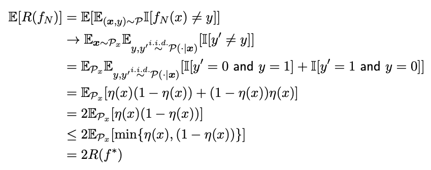
With that it has a strong guarantee that $R(f^*)=0 \Rightarrow\mathbb{E}[R(f_N)]\rightarrow 0$ Thus NNC is very close to optimal solution, the problem is how to defined the distance